I. Introduction:

\(\bullet\) This system contains three generating units with a load demand of 850 MW. Some researchers could evaluate their proposed optimization algorithms with different load demands.
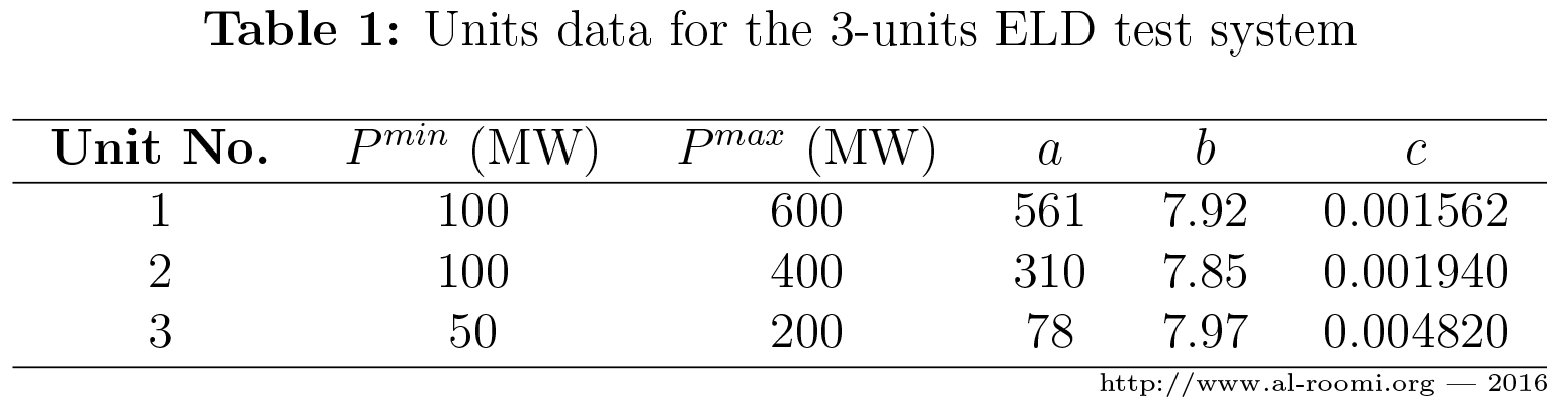
\(\bullet\) The fuel-cost function of this test system is modeled using the quadratic cost function as follows:

\(C_i\left(P_i\right) = a_i + b_i P_i + c_i P^2_i \) .......... \((1)\)

   where \(a_i\), \(b_i\), and \(c_i\) are the function coefficients and tabulated in Table 1.

\(\bullet\) In [1], there are two alternative scenarios regarding this system:
\(\ \ \ \rhd\) The coefficients of the first unit (i.e., \(a_1\), \(b_1\), and \(c_1\)) are respectively 459, 6.48, and 0.00128. Thus, the cost function of the first unit is:

\(C_1\left(P_1\right) = 459 + 6.48 P_1 + 0.00128 P^2_1\) .......... \((2)\)

\(\ \ \ \rhd\) The network losses are modeled as follows:

\(P_L = 0.00003 P^2_1 + 0.00009 P^2_2 + 0.00012 P^2_3\) .......... \((3)\)

   Eq.(3) can be generalized by using Kron's loss formula as follows:

\(P_L = \sum_{i=1}^{n} \sum_{j=1}^{n} P_i B_{ij} P_j + \sum_{i=1}^{n} B_{0i} P_i + B_{00}\) .......... \((4)\)

   where \(B_{ij}\), \(B_{0i}\), and \(B_{00}\) are called loss coefficients (or just B-coefficients) and listed below [15]:

\(B_{ij}=\begin{bmatrix}
0.00003 & 0 & 0\\
0 & 0.00009 & 0\\
0 & 0 & 0.00012
\end{bmatrix}\)

\(B_{0i} = \left[0, 0, 0\right]\)

\(B_{00} = 0\)

   In [2], these \(B_{ij}\), \(B_{0i}\), and \(B_{00}\) are presented as follows:

\(B_{ij}=\begin{bmatrix}
0.0002940 & 0.0000901 & -0.0000507\\
0.0000901 & 0.0005210 & 0.0000953\\
-0.0000507 & 0.0000953 & 0.0006760
\end{bmatrix}\)
\(B_{0i} = \left[0.01890, -0.00342, -0.007660\right]\)
\(B_{00} = 0.40357\)

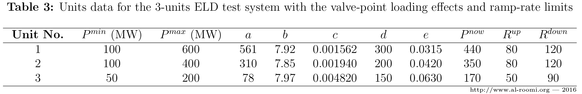
\(\bullet\) If the valve-point loading effects are considered, then (1) becomes:

\(C_i\left(P_i\right) = a_i + b_i P_i + c_i P^2_i + \left|d_i \times \sin\left[e_i \times \left(P_i^{min} - P_i\right) \right]\right|\) .......... \((5)\)

   where \(d_i\) and \(e_i\) are the coefficients of the valve-point loading effects. Thus, Table 1 is expanded to Table 2.

\(\bullet\) The valve-point loading effects can be relaxed if either \(d\) or \(e\) of all units are set to zero.
\(\bullet\) In [16], the ramp-rate limits are modeled as constraints in the design function, so the feasible search space of each unit is determined through the following equation:

\(\text{max}\left(P_i^{min},P_i^{now}-R_i^{down}\right) \leqslant P_i^{new} \leqslant \text{min}\left(P_i^{max},P_i^{now}+R_i^{up}\right)\) .......... \((6)\)

   where \(P_i^{now}\) and \(P_i^{new}\) are respectively the existing and new power output of the \(i\)th generator. \(R_i^{down}\) and \(R_i^{up}\) are respectively the downward and upward ramp-rate limits.
\(\bullet\) Therefore, Table 2 should also be modified to Table 3 if the researcher wants to incorporate all these constraints \(\rightarrow\) Actually, it is based on the comparison criteria used to evaluate the performance of the researcher proposed optimization algorithm with others reported in the literature, because the researcher cannot consider valve-point loading effects, network losses, and/or ramp-rate limits if the other studies used simple model as that given in (1).

\(\bullet\) With using transmission losses given in equation (3), the NOx emission-rates can be modeled in this system as follows [6]:

\(E_{NOx} = \sum_{i=1}^n \left(\alpha_i + \beta_i P_i + \gamma_i P^2_i \right)\) .......... \((7)\)

   where \(\alpha_i\), \(\beta_i\), and \(\gamma_i\) are the coefficients of the \(i\)th unit NOx emission characteristics. Thus, Table 3 is expanded to Table 4.

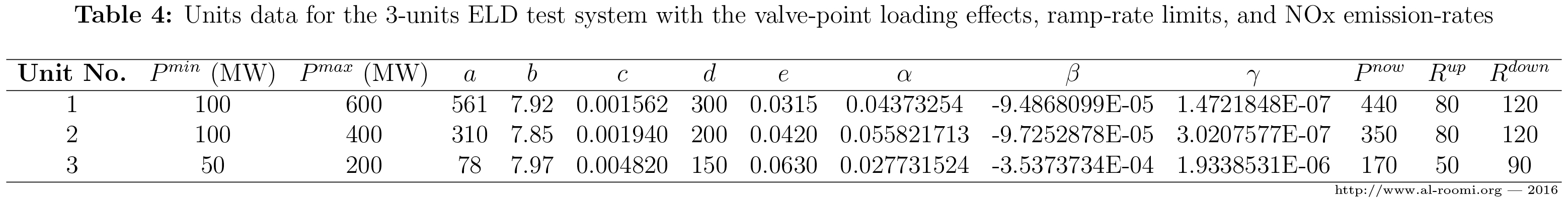
\(\bullet\) Please, note that \(P^{min}_1=150 \text{ MW}\) in some studies, like [1], [6]. Thus, IT IS IMPORTANT to consider this modification based on the studies selected to be compared with your proposed optimization algorithm.

II. Files:

\(\bullet\) System Data (Text Format) [Download]

III. Citation Policy:

If you publish material based on databases obtained from this repository, then, in your acknowledgments, please note the assistance you received by using this repository. This will help others to obtain the same data sets and replicate your experiments. We suggest the following pseudo-APA reference format for referring to this repository:

Ali R. Al-Roomi (2016). Economic Load Dispatch Test Systems Repository [https://www.al-roomi.org/economic-dispatch]. Halifax, Nova Scotia, Canada: Dalhousie University, Electrical and Computer Engineering.

Here is a BiBTeX citation as well:

@MISC{Al-Roomi2016,
author = {Ali R. Al-Roomi},
title = {{Economic Load Dispatch Test Systems Repository}},
year = {2016},
address = {Halifax, Nova Scotia, Canada},
institution = {Dalhousie University, Electrical and Computer Engineering},
url = {https://www.al-roomi.org/economic-dispatch}
}

IV. References (Some selected papers that use this test system):

[1] K. Y. L. J. H. Park, Y.S. Kim, I. K. Eom, “Economic Load Dispatch for Piecewise Quadratic Cost Function Using Hopfield Neural Network,” IEEE Trans. Power Syst., vol. 8, no. 3, pp. 1030–1038, Aug. 1993.
[2] David C. Walters and G. B. Sheble, “Genetic Algorithm Solution of Economic Dispatch with Valve Point Loading,” IEEE Trans. Power Syst., vol. 8, no. 3, pp. 1325–1332, Aug. 1993.
[3] H.-T. Yang, P. Yang, and C.-L. Huang, “Evolutionary Programming Based Economic Dispatch for Units with Non-Smooth Fuel Cost Functions,” IEEE Trans. Power Syst., vol. 11, no. 1, pp. 112–118, Feb. 1996.
[4] C.-T. Su and C.-T. Lin, “New Approach with a Hopfield Modeling Framework to Economic Dispatch,” IEEE Trans. Power Syst., vol. 15, no. 2, pp. 541–545, May 2000.
[5] N. Sinha, R. Chakrabarti, and P. K. Chattopadhyay, “Evolutionary Programming Techniques for Economic Load Dispatch,” IEEE Trans. Evol. Comput., vol. 7, no. 1, pp. 83–94, Feb. 2003.
[6] H. C. S. Rughooputh and R. T. F. A. King, “Environmental/Economic Dispatch of Thermal Units Using an Elitist Multiobjective Evolutionary Algorithm,” in IEEE International Conference on Industrial Technology, 2003 (ICIT 2003), 2003, vol. 1, pp. 48–53.
[7] J.-B. Park, K.-S. Lee, J.-R. Shin, and K. Y. Lee, “A Particle Swarm Optimization for Economic Dispatch With Nonsmooth Cost Functions,” IEEE Trans. Power Syst., vol. 20, no. 1, pp. 34–42, Feb. 2005.
[8] D. Liu and Y. Cai, “Taguchi Method for Solving the Economic Dispatch Problem With Nonsmooth Cost Functions,” IEEE Trans. Power Syst., vol. 20, no. 4, pp. 2006–2014, Nov. 2005.
[9] J. S. Alsumait, J. K. Sykulski, and A. K. Al-Othman, “A Hybrid GA-PS-SQP Method to Solve Power System Valve-Point Economic Dispatch Problems,” Appl. Energy, vol. 87, no. 5, pp. 1773–1781, Nov. 2010.
[10] S. Duman, U. Güvenç, and N. Yörükeren, “Gravitational Search Algorithm for Economic Dispatch with Valve-Point Effects,” Int. Rev. Electr. Eng., vol. 5, no. 6, pp. 2890–2895, 2010.
[11] A. Bhattacharya and P. K. Chattopadhyay, “Hybrid Differential Evolution With Biogeography-Based Optimization for Solution of Economic Load Dispatch,” IEEE Trans. Power Syst., vol. 25, no. 4, pp. 1955–1964, Nov. 2010.
[12] Z. Mohammed and J. Talaq, “Economic Dispatch by Biogeography Based Optimization Method,” in 2011 International Conference on Signal, Image Processing and Applications, 2011, pp. 161–165.
[13] B. Mallikarjuna, M. T. Student, K. H. Reddy, and O. Hemakesavulu, “Economic Load Dispatch Problem with Valve – Point Effect Using a Binary Bat Algorithm,” ACEEE Int. J. Electr. Power Eng., vol. 4, no. 3, pp. 33–38, Nov. 2013.
[14] S. Lu, S. Lou, Y. Wu, and X. Yin, “Power System Economic Dispatch Under Low-Carbon Economy with Carbon Capture Plants Considered,” IET Gener. Transm. Distrib., vol. 7, no. 9, pp. 991–1001, Apr. 2013.
[15] MostafaModiri-Delshad, S. H. A. Kaboli, E. Taslimi, J. Selvaraj, and N. A. Rahim, “An Iterated-Based Optimization Method for Economic Dispatch in Power System,” in 2013 IEEE Conference on Clean Energy and Technology (CEAT), 2013, pp. 88–92.
[16] N. Singh and Y. Kumar, “Economic Load Dispatch with Valve Point Loading Effect and Generator Ramp Rate Limits Constraint using MRPSO,” Int. J. Adv. Res. Comput. Eng. Technol., vol. 2, no. 4, pp. 1472–1477, Apr. 2013.
[17] K. Zare and T. G. Bolandi, “Modified Iteration Particle Swarm Optimization Procedure for Economic Dispatch Solving with Non-Smooth and Non-Convex Fuel Cost Function,” in 3rd IET International Conference on Clean Energy and Technology (CEAT) 2014, 2014, pp. 1–6.
[18] K. P. S. Parmar and B. Khokhar, “Oppositional Biogeography-Based Optimization for Solving Economic Dispatch Problems : An Efficient Method,” in International Conference on Advances in Computer Engineering & Applications (ICACEA-2014) at IMSEC,GZB, 2014, pp. 53–58.
[19] T. H. Khoa, P. M. Vasant, M. S. B. Singh, and V. N. Dieu, “Solving Economic Dispatch Problem with Valve-Point Effects Using Swarm-Based Mean-Variance Mapping Optimization (MVMO),” Cogent Eng., vol. 2, no. 1, pp. 1–18, Aug. 2015.