Wednesday, 24 June 2015 11:08
Parent Category: Unconstrained
Category: n-Dimensions
Hits: 7344
Print
Email

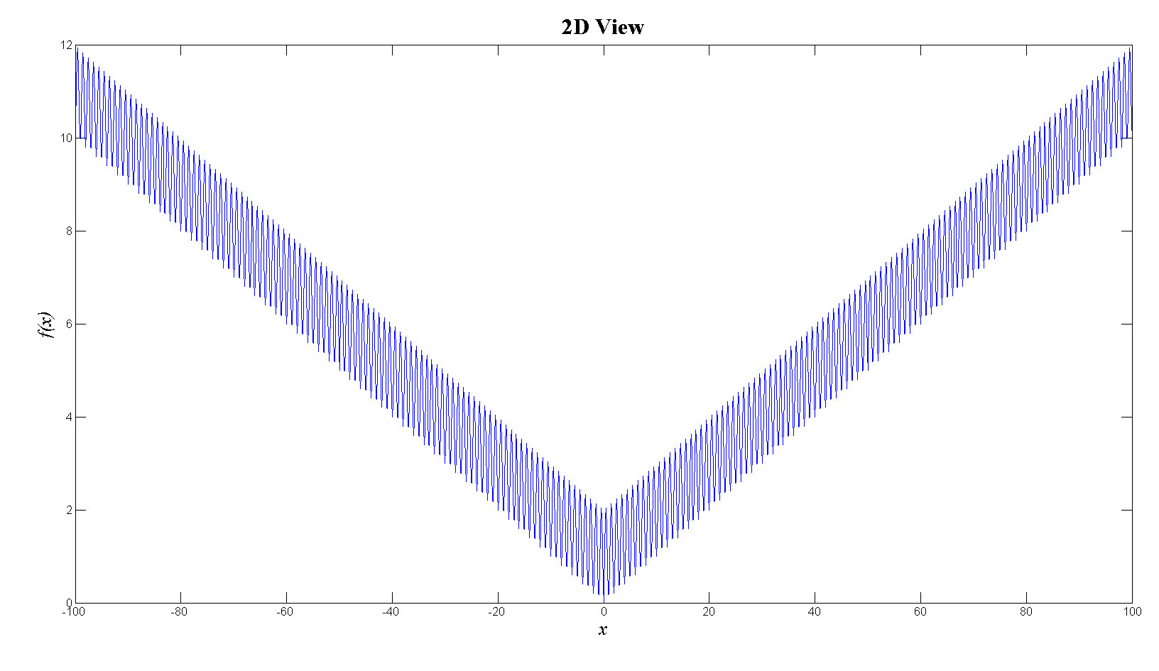
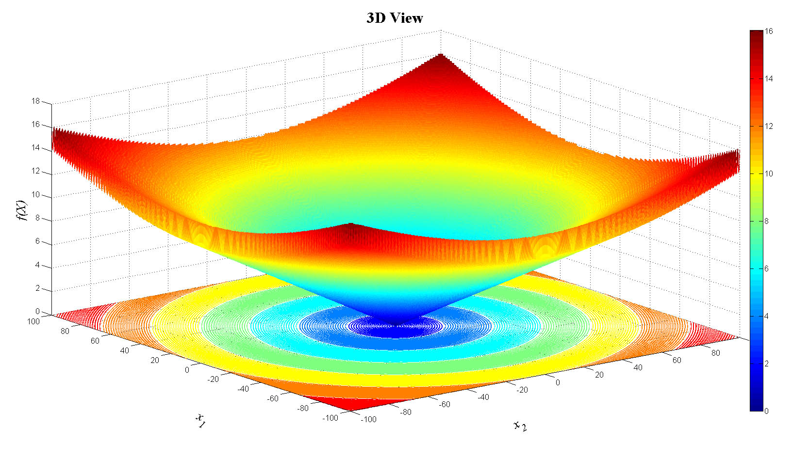
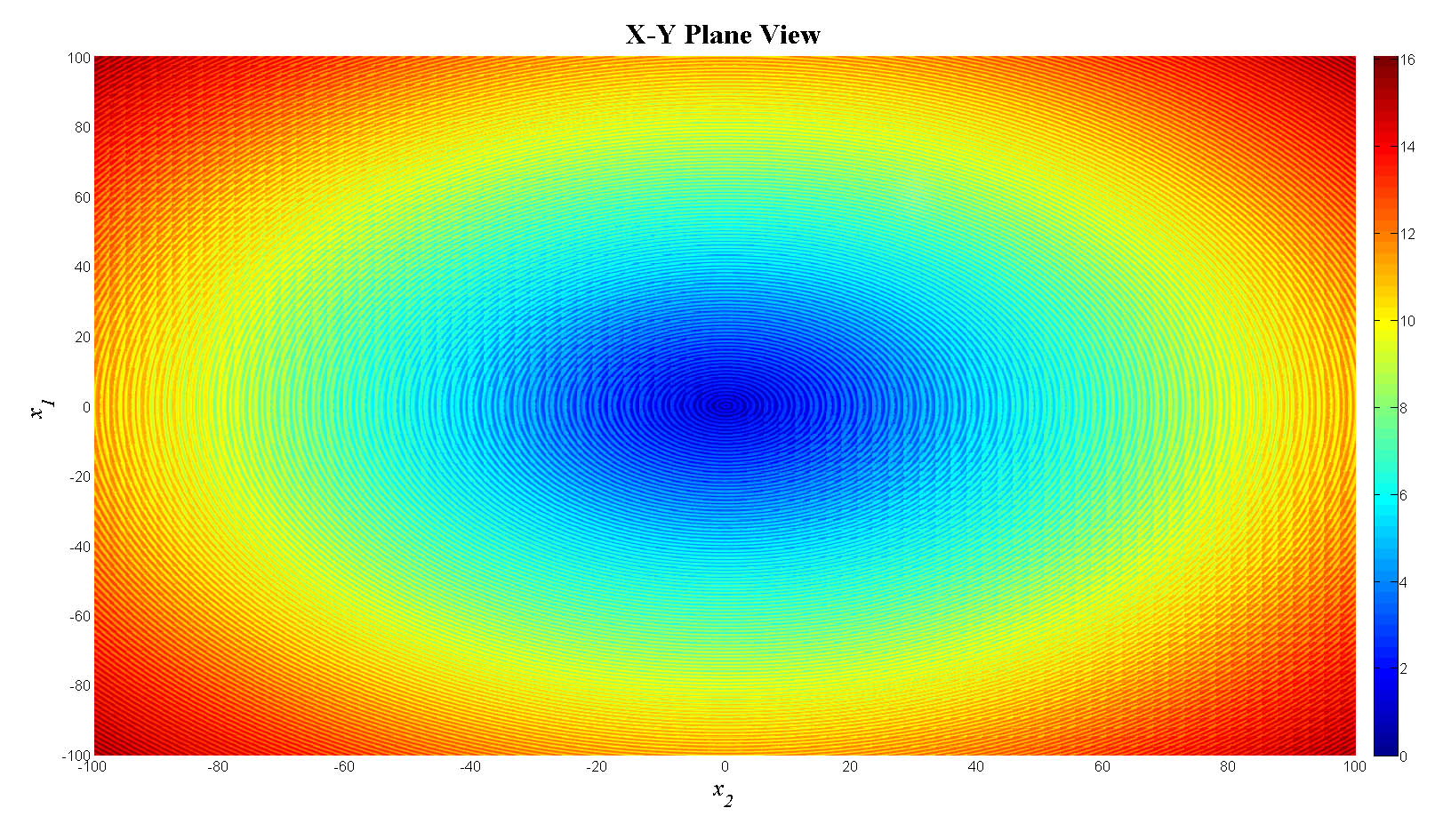
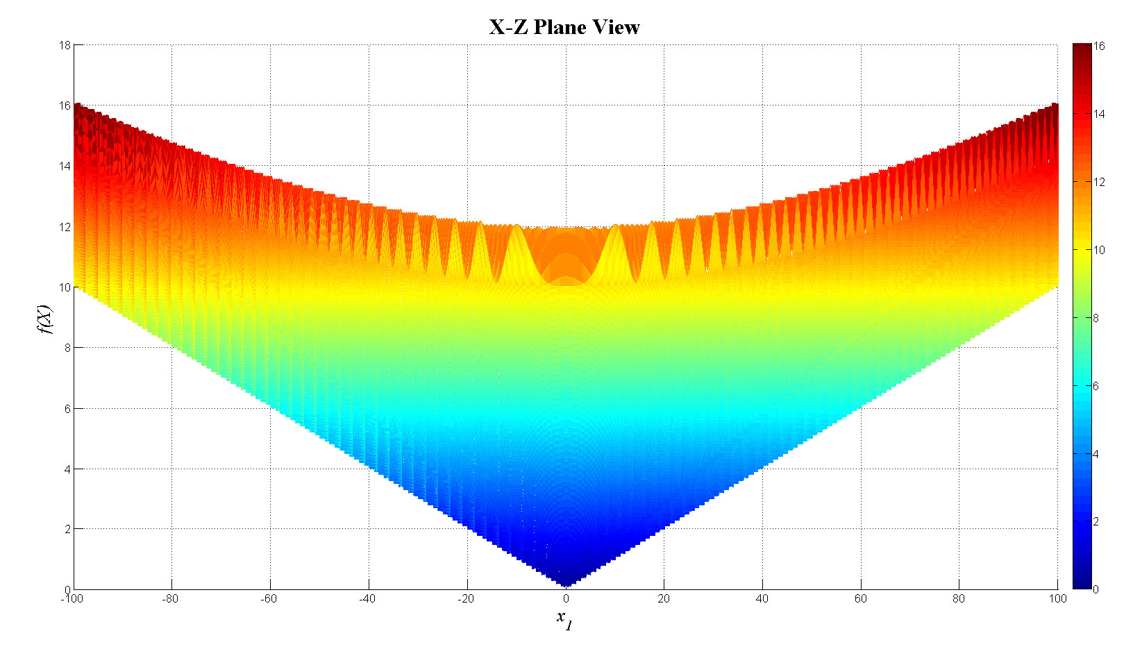
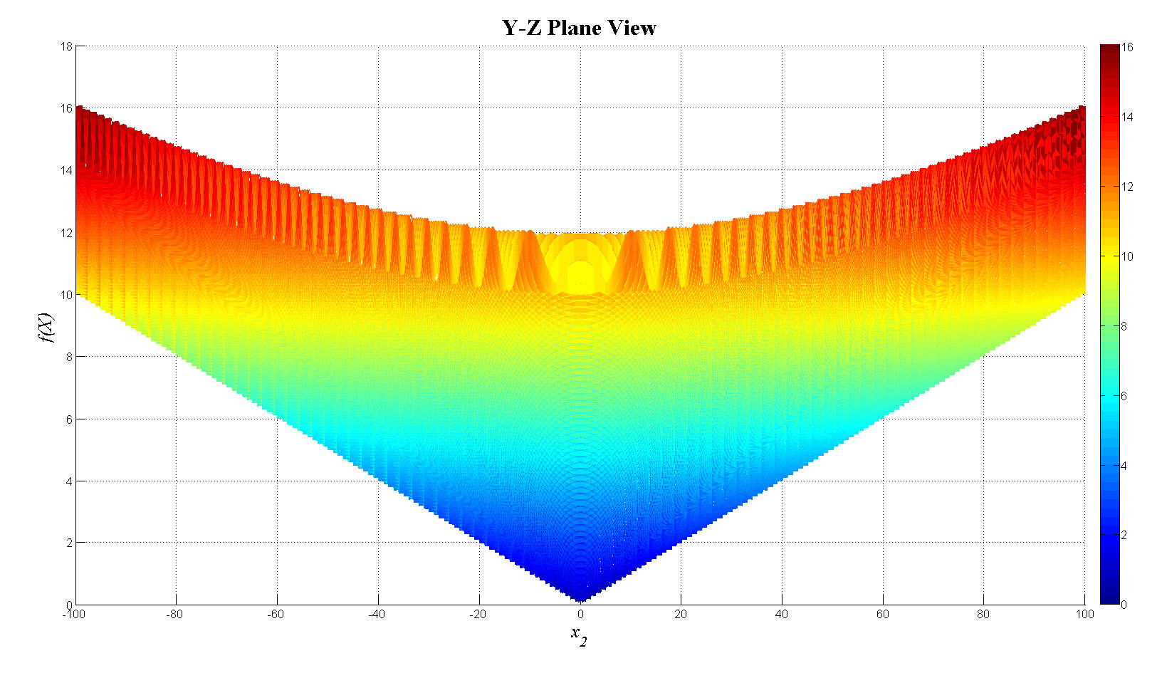
Salomon's Function

I. Mathematical Expression:

$$f(X)=1-\cos\left(2\pi \left \| x \right \|\right)+0.1\left \| x \right \|$$

where:

$\bullet$ $\left \| x \right \|=\sqrt{\sum_{i=1}^{n}x^2_i}$

$\bullet$ $-100\leq x_i\leq 100$ , $i=1,2,\cdots,n$

$\bullet$ $f_{min}(X^*)=0$

$\bullet$ $x^*_i=0$

II. Citation Policy:

If you publish material based on databases obtained from this repository, then, in your acknowledgments, please note the assistance you received by using this repository. This will help others to obtain the same data sets and replicate your experiments. We suggest the following pseudo-APA reference format for referring to this repository:

Ali R. Al-Roomi (2015). Unconstrained Single-Objective Benchmark Functions Repository [https://www.al-roomi.org/benchmarks/unconstrained]. Halifax, Nova Scotia, Canada: Dalhousie University, Electrical and Computer Engineering.

Here is a BiBTeX citation as well:

@MISC{Al-Roomi2015,
author = {Ali R. Al-Roomi},
title = {{Unconstrained Single-Objective Benchmark Functions Repository}},
year = {2015},
address = {Halifax, Nova Scotia, Canada},
institution = {Dalhousie University, Electrical and Computer Engineering},
url = {https://www.al-roomi.org/benchmarks/unconstrained}
}

III. 2&3D-Plots:

IV. Controllable 3D Model:

- In case you want to adjust the rendering mode, camera position, background color or/and 3D measurement tool, please check the following link

- In case you face any problem to run this model on your internet browser (it does not work on mobile phones), please check the following link

V. MATLAB M-File:

% Salomon's Function
% Range of initial points: -100 <= xj <= 100 , j=1,2,...,n
% Global maxima: (x1,x2,...,xn)=0
% f(X)=0
% Coded by: Ali R. Alroomi | Last Update: 07 June 2015 | www.al-roomi.org
 
clear
clc
warning off
   
x1min=-100;
x1max=100;
x2min=-100;
x2max=100;
R=1500; % steps resolution
x1=x1min:(x1max-x1min)/R:x1max;
x2=x2min:(x2max-x2min)/R:x2max;
 
for j=1:length(x1)
    
    % For 1-dimensional plotting
    x_norm1=sqrt(x1(j)^2);
    f1(j)=1-cos(2*pi*x_norm1)+0.1*x_norm1;
    
    % For 2-dimensional plotting
    for i=1:length(x2)
        x_norm2=sqrt(x1(j)^2+x2(i)^2);
        fn(i)=1-cos(2*pi*x_norm2)+0.1*x_norm2;
    end
    
    fn_tot(j,:)=fn;
 
end
 
figure(1)
plot(x1,f1);set(gca,'FontSize',12);
xlabel('x','FontName','Times','FontSize',20,'FontAngle','italic');
ylabel('f(x)','FontName','Times','FontSize',20,'FontAngle','italic');
title('2D View','FontName','Times','FontSize',24,'FontWeight','bold');
 
figure(2)
meshc(x1,x2,fn_tot);colorbar;set(gca,'FontSize',12);
xlabel('x_2','FontName','Times','FontSize',20,'FontAngle','italic');
set(get(gca,'xlabel'),'rotation',25,'VerticalAlignment','bottom');
ylabel('x_1','FontName','Times','FontSize',20,'FontAngle','italic');
set(get(gca,'ylabel'),'rotation',-25,'VerticalAlignment','bottom');
zlabel('f(X)','FontName','Times','FontSize',20,'FontAngle','italic');
title('3D View','FontName','Times','FontSize',24,'FontWeight','bold');
 
figure(3)
mesh(x1,x2,fn_tot);view(0,90);colorbar;set(gca,'FontSize',12);
xlabel('x_2','FontName','Times','FontSize',20,'FontAngle','italic');
ylabel('x_1','FontName','Times','FontSize',20,'FontAngle','italic');
zlabel('f(X)','FontName','Times','FontSize',20,'FontAngle','italic');
title('X-Y Plane View','FontName','Times','FontSize',24,'FontWeight','bold');
 
figure(4)
mesh(x1,x2,fn_tot);view(90,0);colorbar;set(gca,'FontSize',12);
xlabel('x_2','FontName','Times','FontSize',20,'FontAngle','italic');
ylabel('x_1','FontName','Times','FontSize',20,'FontAngle','italic');
zlabel('f(X)','FontName','Times','FontSize',20,'FontAngle','italic');
title('X-Z Plane View','FontName','Times','FontSize',24,'FontWeight','bold');
 
figure(5)
mesh(x1,x2,fn_tot);view(0,0);colorbar;set(gca,'FontSize',12);
xlabel('x_2','FontName','Times','FontSize',20,'FontAngle','italic');
ylabel('x_1','FontName','Times','FontSize',20,'FontAngle','italic');
zlabel('f(X)','FontName','Times','FontSize',20,'FontAngle','italic');
title('Y-Z Plane View','FontName','Times','FontSize',24,'FontWeight','bold');